Distance matrix

Utility for calculating distance matrices at, in between, or excluding variants.

Usage

DistMat(
  fwd,
  bck,
  type = "raw",
  M = NULL,
  beta.theta.opts = NULL,
  nthreads = min(parallel::detectCores(logical = FALSE), fwd$to_recipient -
    fwd$from_recipient + 1)
)

Arguments

fwd: a forward table as returned by MakeForwardTable() and propagated to a target variant by Forward(). Must be at the same variant as bck (unless bck is in "beta-theta space" in which case if must be downstream ... see Backward() for details).
bck: a backward table as returned by MakeBackwardTable() and propagated to a target variant by Backward(). Must be at the same variant as fwd (unless bck is in "beta-theta space" in which case if must be downstream ... see Backward() for details).
type: a string; must be one of "raw", "std" or "minus.min". See Details.
M: a pre-existing matrix into which to write the distances. This can yield substantial speed up but requires special attention, see Details.
beta.theta.opts: a list; see Details.
nthreads: the number of CPU cores to use. By default no parallelism is used. By default uses the parallel package to detect the number of physical cores.

Value

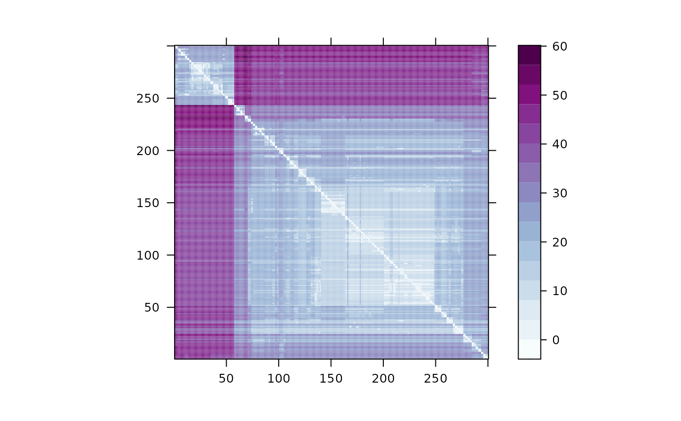
A matrix of distances. The $(j,i)$-th element of of the returned matrix is the inferred distance $d_{ji}$ to haplotype $j$ from haplotype $i$ at the current variant. Each column encodes the output of an independent HMM: in column $i$, haplotype $i$ is taken as the observed recipient haplotype and painted as a mosaic of the other $N-1$ haplotypes. Hence, the distances are asymmetric.

If you wish to plot this matrix or perform clustering, you may want to symmetrize the matrix first.

Details

This computes a local probability or distance matrix based on the forward and backward tables at a certain variant. The default usage is provide forward and backward tables at the same variant $l$ so that the $(j,i)$-th element of of the returned matrix is the inferred distance $d_{ji}$ between haplotypes $j$ and $i$ at the current variant, $l$, of the two tables given the haplotypes observed (over the whole sequence).

In particular,

$$d_{ji} = -log(p_{ji})$$

where $p_{ji}$ is the posterior marginal probability that $j$ is coped by $i$ at the current variant of the two tables, $l$, given the haplotypes observed (over the whole sequence).

By convention, $d_{ii} = 0$ for all $i$.

The above is returned when the type argument is "raw" (the default). However, for convenience, a user may change the type argument to "std" in order for the distances to be mean and variance normalized before returning. Changing type to "minus.min" will subtract the min distance in each column from that column before returning (this is the default in RELATE, see bottom of the RELATE paper Supplement Page 7 (Speidel et al, 2019)).

This function also allows users to calculate distance matrices in between variants and also to calculate matrices that exclude a set of consecutive variants by passing a backward table in "beta-theta space." If in "beta-theta space", bck$l may be greater than but not equal to fwd$l. beta.theta.opts provides is required in this case to set how much of a recombination distance to propagate each matrix before combining them into distances. See Details below.

Notes on beta.theta.opts

In order to obtain distance matrices between variants fwd$l and bck$l, then bck must be in "beta-theta space", see Backward() for details. This allows the forward and backward tables to be transitioning both tables to some genomic position between fwd$l and bck$l. The precise recombination distance by which each table is propagated can be controlled by passing optional arguments in a list via beta.theta.opts. The recombination distances used can be specified in one of two ways.

Manually. In this case, beta.theta.opts is a list containing two named elements:
- "rho.fwd" $\in (0,1)$ specifies the transition probability rho for propagating the forward table.
- "rho.bck" $\in (0,1)$ specifies the transition probability rho for propagating the backward table.
Implicitly. In this case, beta.theta.opts is a list containing two named elements:

"pars": a kalisParameters object that implicitly defines the recombination distance $\rho^\star$ between fwd$l and bck$l
"bias" $\in (0,1)$. The forward table is propagated a distance of (bias)$\rho^\star$ and the backward table is propagated a distance of (1-bias)$\rho^\star$.

Performance notes

If calculating many posterior probability matrices in succession, providing a pre-existing matrix M that can be updated in-place can dramatically increase speed by eliminating the time needed for memory allocation. Be warned, since the matrix is updated in-place, if any other variables point to the same memory address, they will also be simultaneously overwritten. For example, writing

M <- matrix(0, nrow(fwd$alpha), ncol(fwd$alpha))
P <- M
PostProbs(fwd, bck, M = M)

will update M and P simultaneously.

When provided, M must have dimensions matching that of fwd$alpha. Typically, that is simply $N \times N$ for $N$ haplotypes. However, if kalis is being run in a distributed manner, M will be a $N \times R$ matrix where $R$ is the number of recipient haplotypes on the current machine.

References

Speidel, L., Forest, M., Shi, S., & Myers, S. (2019). A method for genome-wide genealogy estimation for thousands of samples. Nature Genetics, 51(1321–1329).

Examples

# To get the posterior probabilities at, say, variants 100 of the toy data
# built into kalis
data("SmallHaps")
data("SmallMap")

CacheHaplotypes(SmallHaps)
#> Warning: haplotypes already cached ... overwriting existing cache.

rho <- CalcRho(diff(SmallMap))
pars <- Parameters(rho)

fwd <- MakeForwardTable(pars)
bck <- MakeBackwardTable(pars)

Forward(fwd, pars, 100)
Backward(bck, pars, 100)

p <- PostProbs(fwd, bck)
d <- DistMat(fwd, bck)

# \donttest{
plot(d)
#> Warning: device support for raster images unknown, ignoring 'raster=TRUE'

# }

References

Aslett, L.J.M. and Christ, R.R. (2024) "kalis: a modern implementation of the Li & Stephens model for local ancestry inference in R", BMC Bioinformatics, 25(1). Available at: doi:10.1186/s12859-024-05688-8 .
Speidel, L., Forest, M., Shi, S. and Myers, S.R. (2019) "A method for genome-wide genealogy estimation for thousands of samples", Nature Genetics, 51, p. 1321-1329. Available at: doi:10.1038/s41588-019-0484-x .
See also
PostProbs() to calculate the posterior marginal probabilities \(p_{ji}\);
Forward() to propagate a Forward table to a new variant;
Backward() to propagate a Backward table to a new variant.